From B. Klecker et al., On the variability of Suprathermal He+ at 1 AU, 2001

This is a copy of the Venus Tail Rays poster created by M. Hilchenbach which includes data from Gruenwaldt et al., 1997.

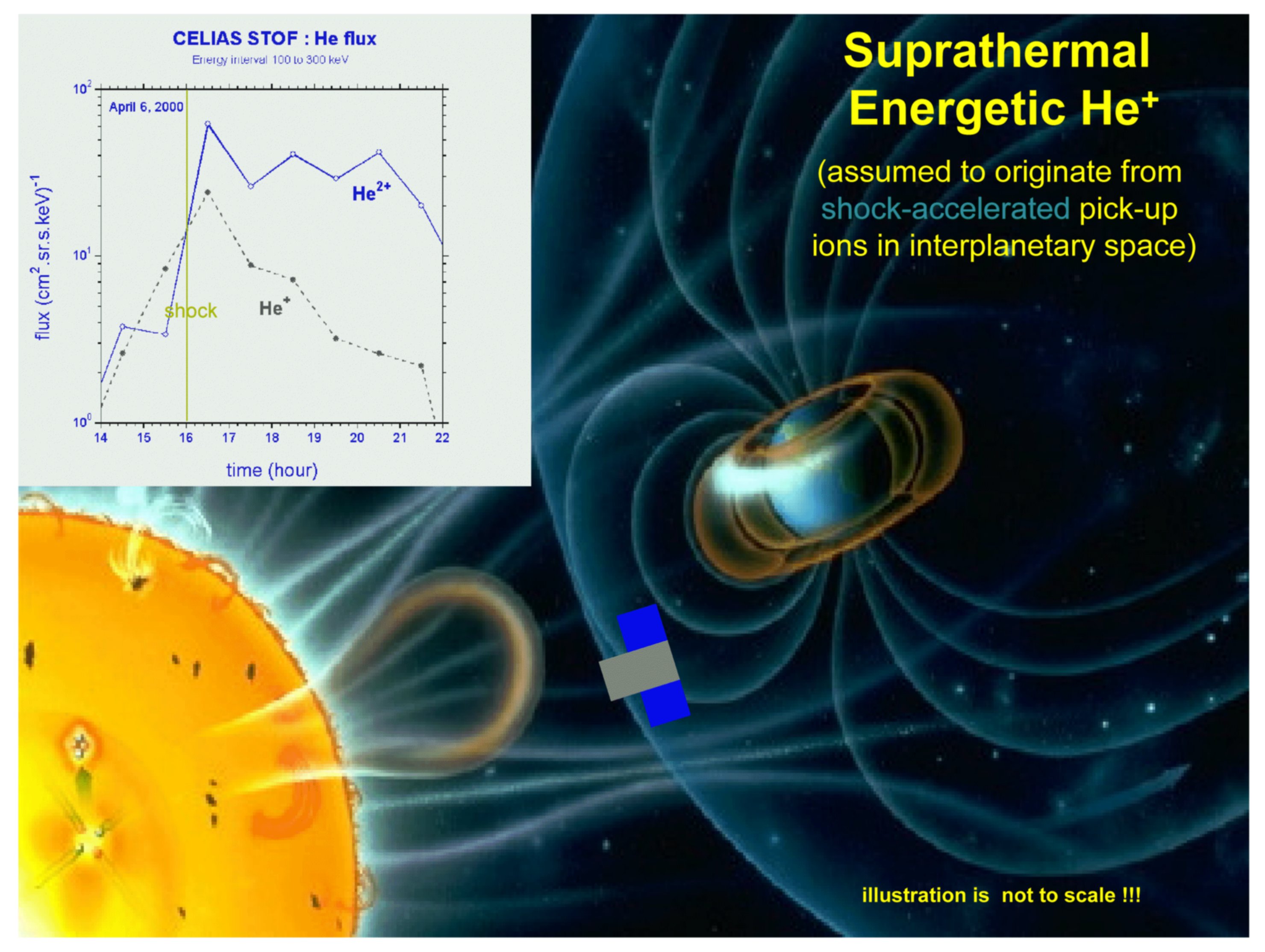
Halo CME of April 6, 2000 observed by SOHO/CELIAS/STOF (by M. Hilchenbach)

Summed spectrum as recorded by CELIAS/MTOF during the interstream period from DOY 304-307, 1998. The solid line shows the result of the 17 parameter Maximum Likelihood Fit.

Within the figure, the thin black line is the result of the raw data from MTOF, the thick black line is the maximum likelihood estimate, and the uncertainty bars have been plotted as well. The uncertainty, at this time, is based on the background counts, WAVE transmission, VMASS transmission efficiency. The preliminary value of ³⁶Ar/³⁸Ar is 5.7 ±0.8 and is determined with the ratio of the areas under the argon peaks from maximum likelihood fit. A fortunate result of this exercise is the clear observation of ³⁵Cl and ³⁷Cl (See the figure above). As far as this author is aware this is the first identification of chlorine within the solar wind.

At the end of April a sequence of large CMEs was observed optically by e.g. SOHO/LASCO: On April 29 (DOY 119) a halo CME, on May 2 (DOY 122) a large CME, and on May 6 (DOY 126) another halo CME. With some delay these events were observed with spacecraft particle experiments of SOHO and ACE at L1. Using data from the CELIAS/STOF sensor onboard SOHO we can study for the first time the energy spectra and the charge state distribution of suprathermal particles in the energy range from 35 to 660 keV/e just above the solar wind distribution and below the low energy flare particle energies.
From top to bottom: the energies of all particles measured by STOF, the energy spectra of He++ and He+ and the charge states of He and Fe for a period of 12 hours during the first CME. - Note that the fluxes are not yet fully calibrated. The He⁺/He⁺⁺ ratio was strongly enhanced during the first halo CME (DOY 120). After a sudden rise it dropped successively to approximately zero. The May 2-3 CME (DOY 122 - 123) shows much less enrichment of He+ in the suprathermal particles. In contrast, in the CME-related solar wind of May 2-3, 1998, a significant enhancement of He+ for an interval of more than 24 hours was found. The mean charge state of Fe of the pre-CME time period is lower than during and after the May 2-3 CME. In the second halo CME (DOY 126 - 128) two kinds of material can be distinguished in time: One with higher charge states of Fe and one with lower. During the time periods with shocks (DOY 121 and 124) and the first halo CME (DOY 120) very hard spectra were observed with spectral indices of about 2 for He⁺⁺. Simultaneously the SWICS and SWIMS instruments on the Advanced Composition Explorer (ACE) observed a most unusual elemental and charge state composition in the solar wind related to the May 2-3 CME: high and low charge states for all elements (e.g., Fe³⁺ to Fe¹⁶⁺), an enhanced ³He/⁴He ratio and a prolongued He⁺ enhancement.

This graph displays the daily average of EUV flux from 260 Å to 340 Å as measured by the SEM sensor from 1996 to 1999.

This CELIAS/MTOF spectrum was accumulated over a three day period (these valuesare uncorrected for efficiencies). The MTOF sensor was set in a mode that was optimized for observing solar wind species with masses above that of sulfur. This is why the peaks for Calcium (mass 40) and Iron (mass 56) are so dominant compared to, for example, Oxygen. In this color version of the figure, the peaks that are simply linedrawn are the elements commonly observed by insitu solar wind experiments: Carbon (mass 12 amu), Oxygen (mass 16 amu), Neon (mass 20), Magnesium (mass 24), Silicon (mass 28), and Iron (mass 56).
The elements and isotopes for which SOHO MTOF has given the first in situ spacecraft solar wind observations are in red. These include the Silicon isotopes (masses 29, 30), the element Phosphorus (mass 31), a Sulfur isotope (mass 34), the element Chlorine (mass 35) and its isotope (mass 37), an Argon isotope (mass 38), the Calcium isotopes (masses 42 and 44), the element Titanium (mass 48), the element Chromium (mass 52) and its isotope (mass 53), the Iron isotope (mass 54, there is also a shoulder for mass 57), the element Manganese (mass 55), the element Nickel (mass 58) and its isotopes (masses 60, 62). [For all but Argon 38, these are the first in situ solar wind observations by any means. There was a measurement of Argon 38 in the Apollo foil experiments, but it had a large uncertainty, and is not frequently quoted by the foil experimenters themselves for solar wind abundance measurements.]
The elements and isotopes that are shaded green are not observed routinely by conventional solar wind experiments. These include the element Nitrogen (mass 14), a Neon isotope (mass 22), the element Sodium (mass 23), the Magnesium isotopes (masses 25, 26), the element Aluminum (mass 27), the Sulfur element (mass 32), the Argon element (mass 36), and the Calcium element (mass 40). Measurements for Sulfur 32 have been made with the Ulysses SWICS experiment, by accumulating over several months of data, and using extensive fitting techniques (it is not really resolved from Iron and Magnesium). Neon 22 and Argon 36 were measured by the Apollo foil experiments. The remainder were first observed in the in situ solar wind by the MTOF prototype sensor, which was launched on WIND about 13 months before SOHO. However, MTOF has a major advantage over its prototype regarding temporal resolution, because of its higher collection power.

On May 6 (DOY 126), 1998 an X-class flare was detected by SOHO/EIT at 0809 UT, and at 0829 UT a very wide and fast CME was seen by SOHO/LASCO. The corresponding suprathermal particle event exhibited a clear velocity dispersion at its onset. The measured energy of each He-particle detected by HSTOF is plotted versus the time of its detection. The corresponding velocity curve is also shown. For a non-relativistic particle of mass m and kinetic energy E, the travel time t along a magnetic field line of length s from near the Sun to L1 is given by t = s * (m/2E)^1/2. We found s = 1.275 ± 0.25 AU. (From K. Bamert, et al., JGR, submitted, 2001).

Solar wind iron isotopic abundances from SOHO/CELIAS/MTOF. From F.M. Ipavich et al., AIP conference proceedings, revised, 2001. See Abstract

Chromium to Iron abundance ratio (as determined by MTOF) for 3 events corresponding to 3 different solar wind flow types. The lighter shaded region represents the 1-sigma range of the meteoritic abundance ratio reported by Grevesse and Sauval (1998). The darker shaded region is the analogous photospheric abundance ratio from the same paper.

Time of Flight spectrum for 50 keV Fe (and contaminants) from the MTOF spare instrument in the MEFISTO accelerator. The peaks are labeled with species and charge state after the foil.

Chromium to Iron Abundance Ratio from MTOF for 3 events corresponding to 3 different solar wind flow types and for the average of three 1-year periods as compared to Grevesse and Sauval (1998)

Enrichment factors of solar wind elements as a function of the Firs Ionization Potential (FIP)

This figure shows the integrated FM2 instrument, consisting of the CTOF (right), MTOF (center back), and STOF (left) sensors, the STOF electronic box and the DPU (back right).

This figure shows the location of the three sensor units of the CELIAS instrument on the SOHO spacecraft: the CTOF (green), MTOF (red), and STOF (blue) sensors.

This figure shows a schematic view of the CTOF sensor.

This figure shows the CTOF FM2 sensor. In the foreground you can see the entrance system consisting of a quadrupol lens (which the red tag at the entrance) and a hemisperical energy analyser in the back. Following that is the TOF section (thick cylinder in the back) and the TOF electronic.

This figure shows simulated data for the CTOF sensor. It is assumed that the post acceleration between the entrance system and the TOF section is turned up to 30 kV. The transmission and the energy resolution of the entrance system are taken from calibrations of the flight model. The performance of the TOF section of the CTOF sensor is derived from measurements of the carbon foil response, the response of the solid-state-detector, and from calibrations of the flight model of the predecessor instrument. For this simulation it is assumed that the solar wind is approaching with 500 km/s and the coronal temperature is 1.2 10⁶K. The assumed total particle density is 10cm^-3. The ionization of the solar wind ions is calculated using the computer code by Arnaud and Rothenflug (1985) with the recent improvements for Fe included (Arnaud 1994). The abundances of the 15 most important elements in the solar wind are derived from measurements of solar energetic particles from Breneman and Stone (1985) for H, He, C, N, O, Ne, Na, Mg, Al, Si, S, Ar, Ca, Fe, and Ni. Furthermore, a He/O ratio of 75 (Bochsler 1986) and a H/He ratio of 25 is used. The CTOF sensor has a special protection against too high count rates, the Proton IDentifier, PID. This analog circuit prevents the CTOF digital electronic from flooding with the high count rates from protons and alpha particles, which are less interesting than the heavier ions. At nominal operations the PID is set to suppress the ⁴He²⁺ peak by 90%, the protons should be suppressed entirely, however ³He²⁺ should come through unattenuated. This feature is included in the simulation. The resulting data is plotted for an integration period for the 24 hours. The lowest contour line in the figure gives the one count level. The one-day integration period corresponds to a SWICS/ULYSSES measurement of more than 100 days. This improvement is due to the better duty cycle, larger geometric factor, and the closer position to the sun of the CTOF/SOHO instrument.

This figure shows a schematic view of the MTOF sensor.

This figure shows the MTOF FM2 sensor with the cover open. There are two openings, one for the proton monitor (on the left), and one for the actual MTOF sensor.

This figure shows a schematic view of the WAVE entrance system. The WAVE consists essentially of three staggered boxes of cylindrical symmetry. High transparency grounded grids cover the front of each of the boxes. The voltages on the back surfaces and on three equally spaced bands along the inside perimeters are such that in each box a constant electric field is generated. The relative sizes of the boxes and the overall geometry are chosen such that ion energy per charge ratios in the range of a factor 5 and entrance angles in the ecliptic of 20° to 70° are accepted. Accepted entrance angles out of the eccliptic are ±30°.

This figure shows the FM2 WAVE entrance system. The solar wind ions enter from the upper right at approximately 45°, pass the first light suppression baffle and continue into the three boxes (white ceramics) of the electrostatic deflection system. Ions with the appropriate energy per charge emerge from the exit grid, the gold platted foil to the right. At the bottom, the black structure is another light suppression baffle. The totel UV-suppression of this entrance system is 2 10^-8.

This figure shows simulated data for the MTOF sensor. It is assumed that the hyperbola of the TOF system (V-MASS) is at 30 kV and no post acceleration/deceleration between the entrance system and the V-MASS is applied. The transmission and the energy pass band of the entrance system are taken from calibrations of the flight model. The ionization efficiencies of particles passing through the carbon foil of V-MASS are taken from calibrations performed at the University of Bern. The mass resolution of the TOF section is derived from several measurements from V-MASS prototypes and the flight model of MTOF. For the simulation of the MTOF sensor response the same data set is used as for the CTOF simulation, however, the data set is enlarged by the isotopic abundances of the various elements. Thus a total of 35 different species is considered. The isotopic abundances are taken from solar system abundances given by Anders and Grevesse (1989) and from terrestrial abundance for Ca were a solar system value was not available. At nominal operations the energy pass band of the entrance system is set to transmit ions from He to Fe only. The shows the resulting mass spectrum in the mass range from 10 to 70 amu for an integration period of 24 hours. The charge exchange of particles passing the carbon foil at the entrance of the V-MASS results in mostly single ionized species, but to a smaller extent also doubly charged ions leave the carbon foil. This effect is also included in the simulation and the respective mass peaks are indicated in figure (dark red). As can be seen contributions from these doubly charged ions to the total signal occur mainly at the mass range from 11 to 15, and will be accounted for in the isotope evaluation using the carbon foil calibrations.

This figure shows a schematic view of the STOF sensor.

This figure shows the STOF FM2 sensor. To the left is the entrance system with the sun shade in front. Following that is the TOF section. The shutter is located between the entrance system and the TOF section with the shutter actuater located at the bottom of the TOF case. The SEM is mounted on the top of the TOF section (the item with the triangular shape). In the black box in the back is the STOF electronic box.

This figure shows simulated data for the STOF sensor. The transmission and the energy resolution of the entrance system are taken from calibrations of the flight model. The performance of the TOF section of the STOF sensor is derived from measurements of the carbon foil response, the response of the solid-state-detector, and from calibrations of the TOF sub-section of the instrument. For the simulation the same abundances for the various elements are used as for the CTOF simulation. However, the ionization temperature varies from element to element (Klecker 1994). For He, C, N, and O the temperature is 2 10⁶K, for Ne up to Si it is 4 10⁶K, for S, Ar, and Ca it is 2.1 10⁶K, and for Fe and Ni it is 2.4 10⁶K. Particles with an energy of 50 keV/nuc are considered in the simulation, which is on the low side of the SEP energy spectrum. The flux of the particles at this energy is 54 10³/cm²-sec-sr-MeV/nuc (Klecker 1994). This corresponds to a quiet day for solar energetic particles. The resulting instrument response is shown in figure for an integration period of 24 hours. Also indicated in figure is the special data compression mechanism used for STOF. Most of the data bins are assigned to the area in mass-mass/charge space where most of the science is anticipated.

This figure shows a schematic diagram of the EUV monitor system.

This is an image of the SEM sensor from the CELIAS Instrument.

This figure shows the solar EUV flux spectrum for quiet (hatched bars) and active (open bars) conditions together with the ionization cross-section of He (in arbitrary units) and the sensitivity of an Al-coated Si-photodiode (in arbitrary units). Also shown are the wavelength ranges of the CDS, SUMER, EIT, and UVCS instruments on SOHO.

This figure shows the basicstructure of the DPU consisting of the sensor interface (SIF), the classification unit (CLU), and the hard core (H/C).

This is the offical SOHO logo.

This is the offical CELIAS Logo

CELIAS team group photo from the 7^th CELIAS Postlaunch Workshop.

CELIAS team group photo from the 8^th CELIAS Postlaunch Workshop.

CELIAS team group photo from the 10^th CELIAS Postlaunch Workshop.

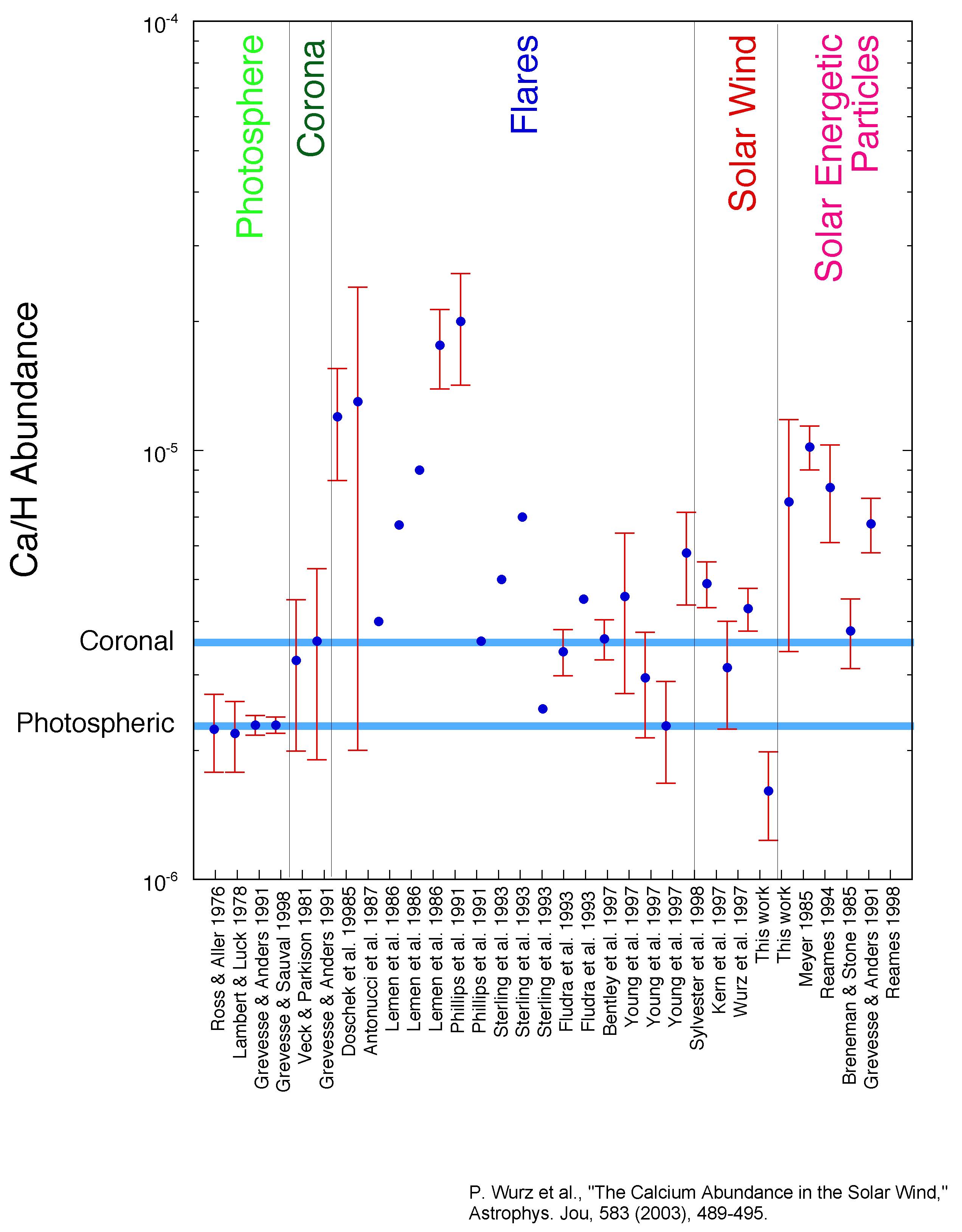
Ca/H Abundance

CELIAS workshop, 26-28 August 2014, MPS Göttingen